


-
In the study of telecommunication system, the variable coefficient (3+1)-dimensional cubic-quintic complex Ginzburg-Landau equation is used as the optical solitons transmission model, which not only explains the physical meaning of the existing model with quintic terms, but also has more nonlinear dynamics characteristics of the higher dimensional system than the lower dimensional system. In this paper, the analytical soliton solutions of the (3+1)-dimensional cubic-quintic CGL equations with variable coefficients are obtained by using the modified Hirota method. By selecting certain parameters of the nonlinear coefficients and spectral filtering terms, a special kind of mixed soliton solution is obtained, which has the characteristics of bright soliton, dark soliton and kinked soliton at the same time. Subsequently, the influence of changing the nonlinear, spectral filtering, linear loss parameters and other parameters on the transmission characteristics of solitons is discussed respectively, so as to realize the control of optical solitons, which can not only control the propagation of optical solitons in different forms, but also can realize the adjustment of the amplitude and pulse width of the pulse and control the propagation direction and energy of the pulse for the mixed solitons of a particular form. The research results of high dimensional CGL system in this paper can be applied to nonlinear optical system, ultra-fast optical digital logic system and other different experiments and application fields.
[1] Akhmediev N N, Ankiewicz A, Soto-Crespo J M 1998 JOSA B 15 515
 Google Scholar
[2] Kivshar Y S, Agrawal G 2003 Optical Solitons: from Fibers to Photonic Crystals (USA: Academic Press)
[3] Wang L, Luan Z, Zhou Q, Biswas A, Alzahrani A K, Liu W 2021 Nonlinear Dyn. 104 629
Google Scholar
[4] Wang L L, Liu W J 2020 Chin. Phys. B 29 070502
Google Scholar
[5] Wang T Y, Zhou Q, Liu W J 2022 Chin. Phys. B 31 020501
Google Scholar
[6] Liu Y K, Li B 2017 Chin. Phys. Lett. 34 010202
Google Scholar
[7] Yan Y Y, Liu W J 2021 Chin. Phys. Lett. 38 094201
Google Scholar
[8] Zhang X M, Qin Y H, Ling L M, Zhao L C 2021 Chin. Phys. Lett. 38 090201
Google Scholar
[9] Liu W, Shi T, Liu M, Wang Q, Liu X, Zhou Q, Wei Z 2021 Opt. Express 29 29402
Google Scholar
[10] Ma G, Zhao J, Zhou Q, Biswas A, Liu W 2021 Nonlinear Dyn. 106 2479
Google Scholar
[11] Wazwaz A M 2006 Appl. Math. Lett. 19 1007
Google Scholar
[12] Yan Y, Liu W, Zhou Q, Biswas A 2020 Nonlinear Dyn. 99 1313
Google Scholar
[13] Wang L, Luan Z, Zhou Q, Biswas A, Alzahrani A K, Liu W 2021 Nonlinear Dyn. 104 2613
Google Scholar
[14] Wang H T, Li X, Zhou Q, Liu W J 2023 Chaos Soliton. Fract. 166 112924
Google Scholar
[15] Guan X, Yang H, Meng X, Liu W 2023 Appl. Math. Lett. 136 108466
Google Scholar
[16] Wang H, Zhou Q, Liu W 2022 J. Adv. Res. 38 179
Google Scholar
[17] Liu W, Xiong X, Liu M, Xing X W, Chen H, Ye H, Han J, Wei Z 2022 Appl. Math. Lett. 120 053108
Google Scholar
[18] Liu M, Wu H, Liu X, Wang Y, Lei M, Liu W, Guo W, Wei Z 2021 OEA 4 200029
Google Scholar
[19] Liu X, Zhang H, Liu W 2022 Appl. Math. Model 102 305
Google Scholar
[20] Xu D H, Lou S Y 2020 Acta Phys. Sin. 69 014208
Google Scholar
[21] Li M, Wang B T, Xu T, Shui J J 2020 Acta Phys. Sin. 69 010502
Google Scholar
[22] Wang B, Zhang Z, Li B 2020 Appl. Math. Lett. 37 030501
Google Scholar
[23] Liu W, Yu W, Yang C, Liu M, Zhang Y, Lei M 2017 Nonlinear Dyn. 89 2933
Google Scholar
[24] Zhang J, Yan G 2015 Physica A 440 19
Google Scholar
[25] Yue C, Lu D, Arshad M, Nasreen N, Qian X 2020 Entropy 22 202
Google Scholar
[26] Zhang J, Yan G 2015 Comput. Math. Appl. 70 2904
Google Scholar
[27] Mihalache D, Mazilu D, Lederer F, Leblond H, Malomed B A 2008 Phys. Rev. A 77 033817
Google Scholar
[28] Gui L, Xiao X, Yang C 2013 J. Opt. Soc. Am. B 30 158
Google Scholar
[29] Liu X M, Han X X, Yao X K 2016 Sci. Rep. 6 1
Google Scholar
[30] Hirota R 1971 Phys. Rev. Lett. 27 1192
Google Scholar
[31] Hirota R 1973 J. Math. Phys. 14 805
Google Scholar
-

图 1 亮孤子的具体参数
$ {p_2}(z) $ =${\rm sech}(z)$ ,$ {q_1}(z) $ = 1,$ {r_2}(z) $ =${-{\rm exp}}(z)$ ,$ {b_1} $ = 0.05,$ {b_2} $ = 0.3,$ {c_1} $ = 0.06,$ {c_2} $ = 0.7,$ {d_1} $ = 0.07,$ {d_2} $ = 0.4, y = 1, z = 1,$ {k_1} $ = 0.8,$ {k_2} $ = 0.68,$ {\alpha }= 0.18 $ Figure 1. Specific parameters of bright solitons.
$ {p_2}(z) $ =${\rm sech}(z)$ ,$ {q_1}(z) $ = 1,$ {r_2}(z) $ =${-{\rm exp}}(z)$ ,$ {b_1} $ = 0.05,$ {b_2} $ = 0.3,$ {c_1} $ = 0.06,$ {c_2} $ = 0.7,$ {d_1} $ = 0.07,$ {d_2} $ = 0.4, y = 1, z = 1,$ {k_1} $ = 0.8,$ {k_2} $ = 0.68,$ {\alpha } $ = 0.18.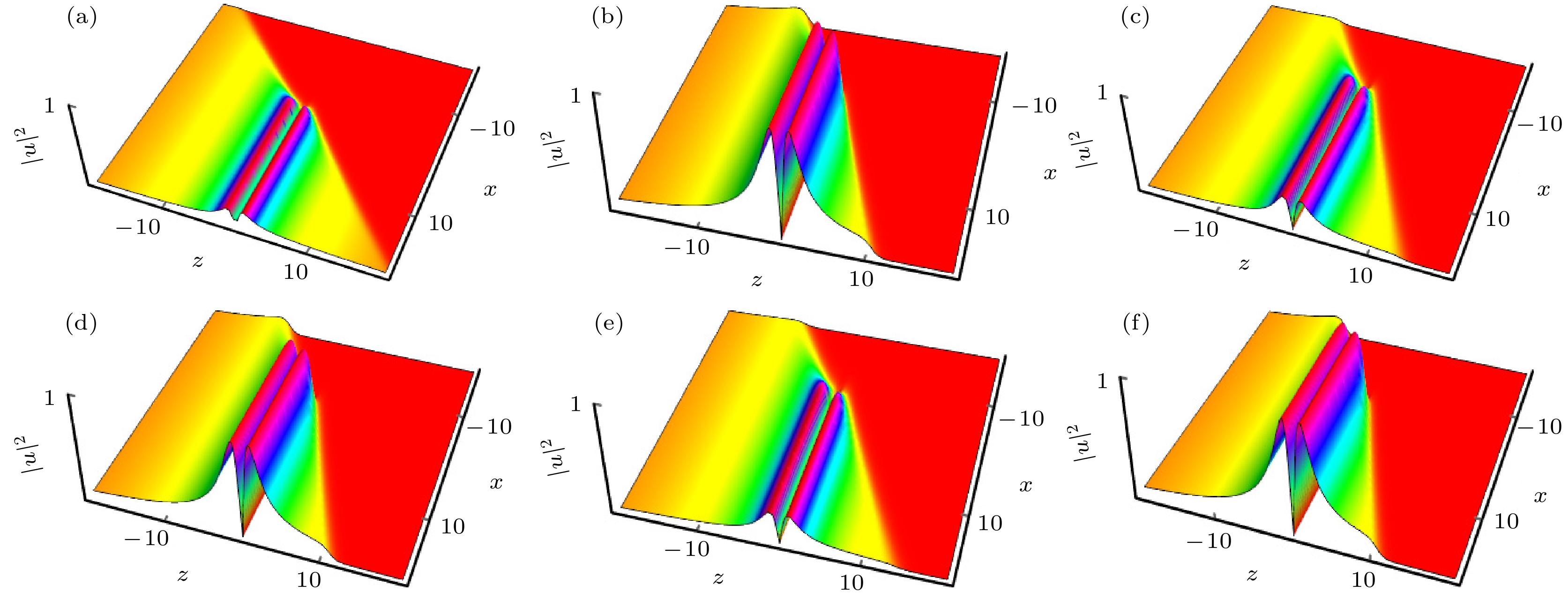
图 5 常数变量对混合孤子形态的影响 (a) b1 = 0.9,
$ {b_2} $ = 0.47,$ {c_1} $ = 0.25,$ {c_2} $ = 0.24,$ {d_1} $ = 0.67,$ {d_2} $ = 0.44; (b)$ {b_1} $ = 0.45,$ {b_2} $ = 0.47,$ {c_1} $ = 0.6,$ {c_2} $ = 0.24,$ {d_1} $ = 0.67,$ {d_2} $ = 0.44; (c)$ {b_1} $ = 0.45,$ {b_2} $ = 0.47,$ {c_1} $ = 0.25,$ {c_2} $ = 0.24,$ {d_1} $ = 0.9,$ {d_2} $ = 0.44; (d)$ {b_1} $ = 0.45,$ {b_2} $ = 0.7,$ {c_1} $ = 0.25,$ {c_2} $ = 0.24,$ {d_1} $ = 0.67,$ {d_2} $ = 0.44; (e)$ {b_1} $ = 0.45,$ {b_2} $ = 0.47,$ {c_1} $ = 0.25,$ {c_2} $ = 0.6,$ {d_1} $ = 0.67,$ {d_2} $ = 0.44; (f)$ {b_1} $ = 0.45,$ {b_2} $ = 0.47,$ {c_1} $ = 0.25,$ {c_2} $ = 0.24,$ {d_1} $ = 0.67,$ {d_2} $ = 0.6, 其余参数为$ {p_2}(z) $ =$0.5{({\rm tanh}z)}^2$ ,$ {q _1}(z) $ = 0.5 z,$ {r _2}(z) $ =${-\rm exp}(z)$ , y = 1, z = 1,$ {k_1} $ = 0.8,$ {k_2} $ =0.68,$ {\alpha } $ = 0.222Figure 5. Effect of constant variable on morphology of mixed soliton. (a)
$ {b_1} $ = 0.9,$ {b_2} $ = 0.47,$ {c_1} $ = 0.25,$ {c_2} $ = 0.24,$ {d_1} $ = 0.67,$ {d_2} $ = 0.44; (b)$ {b_1} $ = 0.45,$ {b_2} $ = 0.47,$ {c_1} $ = 0.6,$ {c_2} $ = 0.24,$ {d_1} $ = 0.67,$ {d_2} $ = 0.44; (c)$ {b_1} $ = 0.45,$ {b_2} $ = 0.47,$ {c_1} $ = 0.25,$ {c_2} $ = 0.24,$ {d_1} $ = 0.9,$ {d_2} $ = 0.44; (d)$ {b_1} $ = 0.45,$ {b_2} $ = 0.7,$ {c_1} $ = 0.25,$ {c_2} $ = 0.24,$ {d_1} $ = 0.67,$ {d_2} $ = 0.44; (e)$ {b_1} $ = 0.45,$ {b_2} $ = 0.47,$ {c_1} $ = 0.25,$ {c_2} $ = 0.6,$ {d_1} $ = 0.67,$ {d_2} $ = 0.44; (f)$ {b_1} $ = 0.45,$ {b_2} $ = 0.47,$ {c_1} $ = 0.25,$ {c_2} $ = 0.24,$ {d_1} $ = 0.67,$ {d_2} $ = 0.6, other parameters$ {p _2}(z) $ =$0.5{({\rm tanh}z)}^2$ ,$ {q _1}(z) $ = 0.5z,$ {r _2}(z) $ =${-\rm exp}(z)$ , y = 1, z = 1,$ {k_1} $ = 0.8,$ {k_2} $ = 0.68,$ {\alpha } $ = 0.222.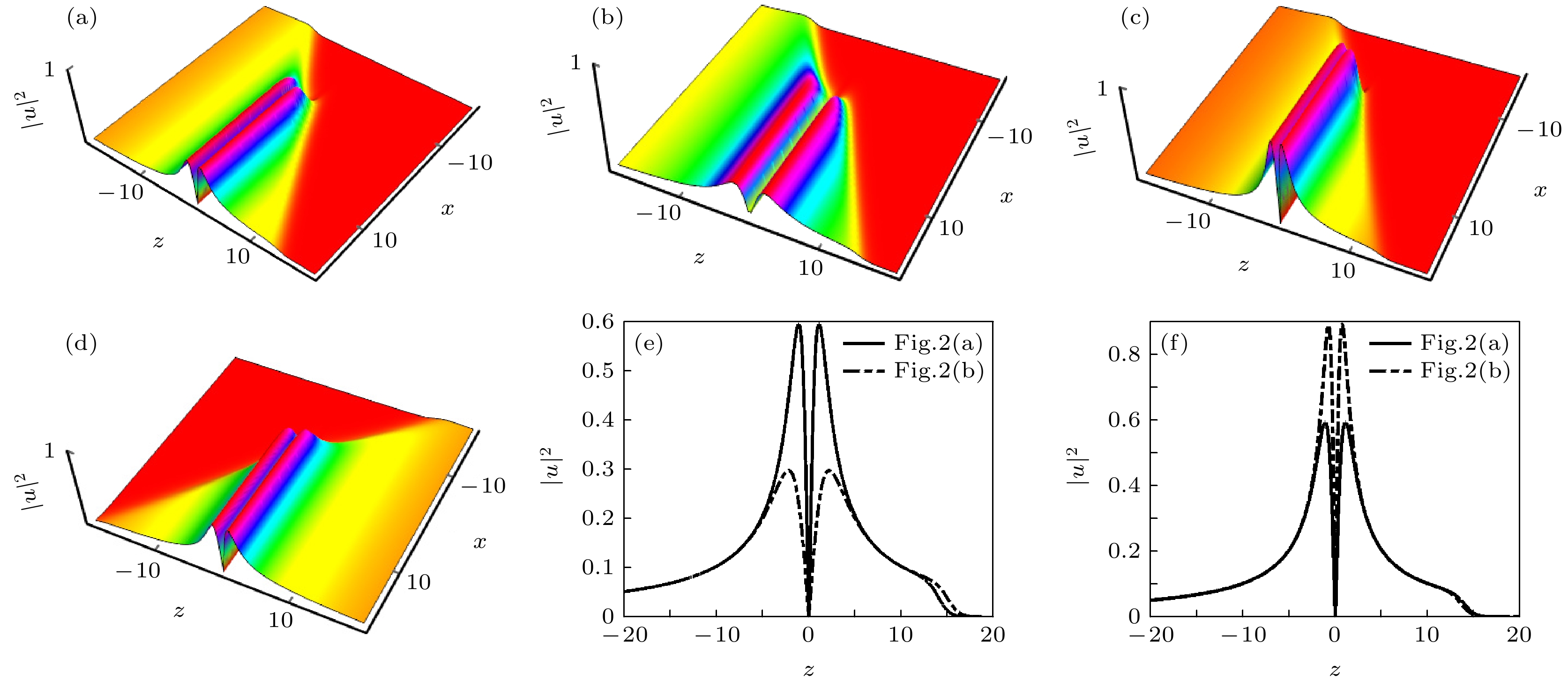
图 2 混合孤子的具体参数及光谱滤波函数对混合孤子形态影响 (a)
$ {p_2}(z) $ =$0.5{({\rm tanh} z)}^2$ ,$ {\alpha} $ = 0.222; (b)$ {p_2}(z) $ = 0.5${[{\rm tanh}(0.5 z)]}^2$ ,$ {\alpha } $ = 0.222; (c)$ {p_2}(z) $ =$0.5{[{\rm tanh}(1.5 z)]}^2$ ,$ {\alpha } $ = 0.222; (d)$ {p_2}(z) $ =$0.5{({\rm tanh}z)}^2$ ,$ {\alpha } $ = 0414, 其余参数$ {q _1}(z) $ = 0.5 z,$ {r _2}(z) $ =${-\rm exp}(z)$ ,$ {b_1} $ = 0.45,$ {b_2} $ = 0.47,$ {c_1} $ = 0.25,$ {c_2} $ = 0.24,$ {d_1} $ = 0.67,$ {d_2} $ =0.44, y = 1, z = 1,$ {k_1} $ = 0.8,$ {k_2} $ = 0.68; (e) x = 0时, 子图(a)和(b)脉冲对比; (f) x = 0时, 子图(a)和(c)脉冲对比Figure 2. Effect of specific parameters of mixed solitons and spectral filtering function on the morphology of mixed solitons. (a)
$ {p_2}(z) $ =$0.5{({\rm tanh}z)}^2$ ,$ {\alpha} $ = 0.222; (b)$ {p_2}(z) $ =$0.5{[{\rm tanh}(0.5 z)]}^2$ ,$ {\alpha } $ = 0.222; (c)$ {p_2}(z) $ =$0.5{[{\rm tanh}(1.5 z)]}^2$ ,$ {\alpha } $ = 0.222; (d)$ {p_2}(z) $ =$0.5{({\rm tanh}z)}^2$ ,$ {\alpha } $ = 0414, other parameters$ {q _1}(z) $ = 0.5 z,$ {r _2}(z) $ =${-\rm exp}(z)$ ,$ {b_1} $ = 0.45,$ {b_2} $ = 0.47,$ {c_1} $ = 0.25,$ {c_2} $ = 0.24,$ {d_1} $ = 0.67,$ {d_2} $ = 0.44, y = 1, z = 1,$ {k_1} $ = 0.8,$ {k_2} $ = 0.68; (e) when x = 0, ulse contrast of panel (a) and (b); (f) when x = 0, pulse contrast of panel (a) and (c).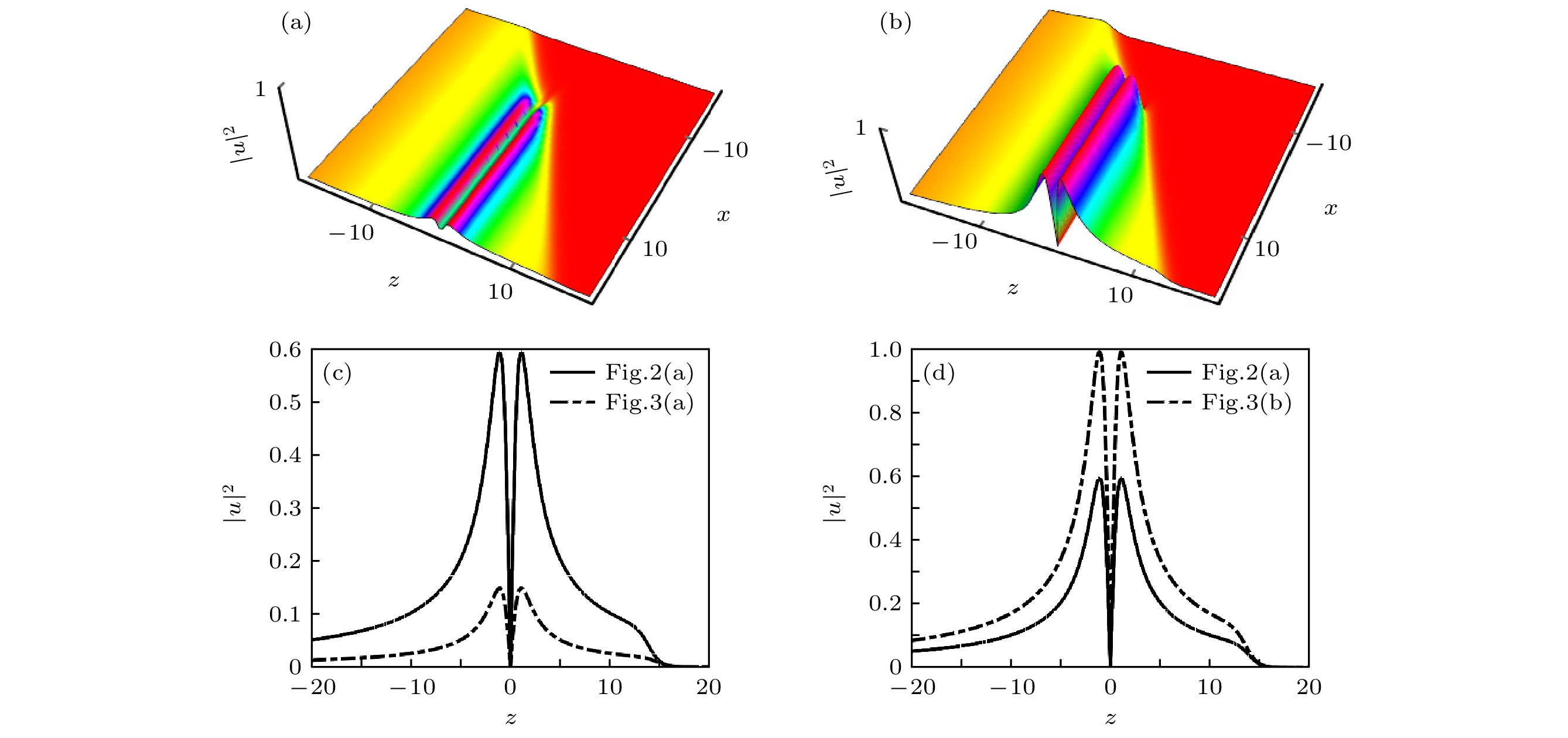
图 3 非线性增益-吸收系数函数对混合孤子形态的影响 (a)
$ {q _1}(z) $ = 2z; (b)$ {q _1}(z) $ = 0.3z, 其余参数$ {p_2}(z) $ =$0.5{({\rm tanh}z)}^2$ ,$ {r _2}(z) $ =${-\rm exp}(z)$ ,$ {b_1} $ = 0.45,$ {b_2} $ = 0.47,$ {c_1} $ = 0.25,$ {c_2} $ = 0.24,$ {d_1} $ = 0.67,$ {d_2} $ = 0.44, y = 1, z = 1,$ {k_1} $ = 0.8,$ {k_2} $ = 0.68,$ {\alpha } $ = 0.222; (c) x = 0时, 图2(a)和图3(a)脉冲对比; (d) x = 0时, 图2(a)和图3(b)脉冲对比Figure 3. Effect of nonlinear gain-absorption coefficient function on the morphology of mixed solitons. (a)
$ {q _1}(z) $ = 2z; (b)$ {q _1}(z) $ = 0.3 z, other parameters$ {p_2}(z) $ =$0.5{({\rm tanh}z)}^2$ ,$ {r _2}(z) $ =${-\rm exp}(z)$ ,$ {b_1} $ = 0.45,$ {b_2} $ = 0.47,$ {c_1} $ = 0.25,$ {c_2} $ = 0.24,$ {d_1} $ = 0.67,$ {d_2} $ = 0.44, y = 1, z = 1,$ {k_1} $ = 0.8,$ {k_2} $ = 0.68,$ {\alpha } $ = 0.222; (c) when x = 0, Fig. 2(a) and Fig. 3(a) pulse contrast; (f) when x = 0, Fig. 2(a) and Fig. 3(b) pulse contrast.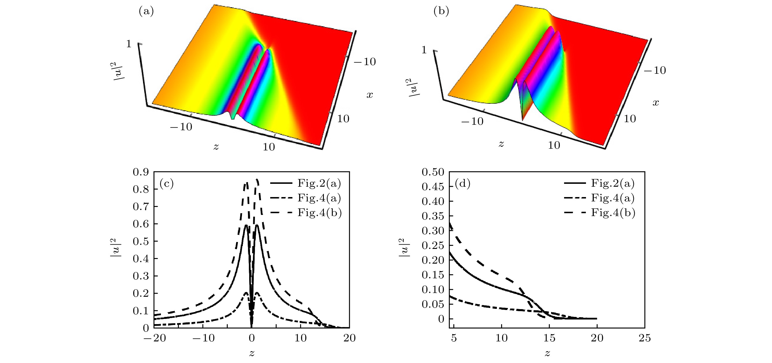
图 4 参数α对混合孤子形态的影响 (a)
$ {\alpha } $ = 0.282; (b)$ {\alpha } $ = 0.182, 其余参数$ {p_2}(z) $ =$0.5{({\rm tanh}z)}^2$ ,$ {q _1}(z) $ = 0.5 z,$ {r _2}(z) $ =${-\rm exp}(z)$ ,$ {b_1} $ = 0.45,$ {b_2} $ = 0.47,$ {c_1} $ = 0.25,$ {c_2} $ = 0.24,$ {d_1} $ = 0.67,$ {d_2} $ = 0.44, y = 1, z = 1,$ {k_1} $ = 0.8,$ {k_2} $ = 0.68; (c) x = 0时, 图2(a)和图4(a), (b)脉冲对比; (d)局部放大图Figure 4. Effect of parameter α on morphology of mixed soliton. (a)
$ {\alpha } $ = 0.282, (b)$ {\alpha } $ = 0.182, other parameters$ {p_2}(z) $ =$0.5{({\rm tanh}z)}^2$ ,$ {q _1}(z) $ = 0.5 z,$ {r _2}(z) $ =${-\rm exp}(z)$ ,$ {b_1} $ = 0.45,$ {b_2} $ = 0.47,$ {c_1} $ = 0.25,$ {c_2} $ = 0.24,$ {d_1} $ = 0.67,$ {d_2} $ = 0.44, y = 1, z = 1,$ {k_1} $ = 0.8,$ {k_2} $ = 0.68; (c) when x = 0, pulse contrast of Fig. 2(a) and Figs. 4(a), (b); (d) partial magnify figure. -
[1] Akhmediev N N, Ankiewicz A, Soto-Crespo J M 1998 JOSA B 15 515
Google Scholar
[2] Kivshar Y S, Agrawal G 2003 Optical Solitons: from Fibers to Photonic Crystals (USA: Academic Press)
[3] Wang L, Luan Z, Zhou Q, Biswas A, Alzahrani A K, Liu W 2021 Nonlinear Dyn. 104 629
Google Scholar
[4] Wang L L, Liu W J 2020 Chin. Phys. B 29 070502
Google Scholar
[5] Wang T Y, Zhou Q, Liu W J 2022 Chin. Phys. B 31 020501
Google Scholar
[6] Liu Y K, Li B 2017 Chin. Phys. Lett. 34 010202
Google Scholar
[7] Yan Y Y, Liu W J 2021 Chin. Phys. Lett. 38 094201
Google Scholar
[8] Zhang X M, Qin Y H, Ling L M, Zhao L C 2021 Chin. Phys. Lett. 38 090201
Google Scholar
[9] Liu W, Shi T, Liu M, Wang Q, Liu X, Zhou Q, Wei Z 2021 Opt. Express 29 29402
Google Scholar
[10] Ma G, Zhao J, Zhou Q, Biswas A, Liu W 2021 Nonlinear Dyn. 106 2479
Google Scholar
[11] Wazwaz A M 2006 Appl. Math. Lett. 19 1007
Google Scholar
[12] Yan Y, Liu W, Zhou Q, Biswas A 2020 Nonlinear Dyn. 99 1313
Google Scholar
[13] Wang L, Luan Z, Zhou Q, Biswas A, Alzahrani A K, Liu W 2021 Nonlinear Dyn. 104 2613
Google Scholar
[14] Wang H T, Li X, Zhou Q, Liu W J 2023 Chaos Soliton. Fract. 166 112924
Google Scholar
[15] Guan X, Yang H, Meng X, Liu W 2023 Appl. Math. Lett. 136 108466
Google Scholar
[16] Wang H, Zhou Q, Liu W 2022 J. Adv. Res. 38 179
Google Scholar
[17] Liu W, Xiong X, Liu M, Xing X W, Chen H, Ye H, Han J, Wei Z 2022 Appl. Math. Lett. 120 053108
Google Scholar
[18] Liu M, Wu H, Liu X, Wang Y, Lei M, Liu W, Guo W, Wei Z 2021 OEA 4 200029
Google Scholar
[19] Liu X, Zhang H, Liu W 2022 Appl. Math. Model 102 305
Google Scholar
[20] Xu D H, Lou S Y 2020 Acta Phys. Sin. 69 014208
Google Scholar
[21] Li M, Wang B T, Xu T, Shui J J 2020 Acta Phys. Sin. 69 010502
Google Scholar
[22] Wang B, Zhang Z, Li B 2020 Appl. Math. Lett. 37 030501
Google Scholar
[23] Liu W, Yu W, Yang C, Liu M, Zhang Y, Lei M 2017 Nonlinear Dyn. 89 2933
Google Scholar
[24] Zhang J, Yan G 2015 Physica A 440 19
Google Scholar
[25] Yue C, Lu D, Arshad M, Nasreen N, Qian X 2020 Entropy 22 202
Google Scholar
[26] Zhang J, Yan G 2015 Comput. Math. Appl. 70 2904
Google Scholar
[27] Mihalache D, Mazilu D, Lederer F, Leblond H, Malomed B A 2008 Phys. Rev. A 77 033817
Google Scholar
[28] Gui L, Xiao X, Yang C 2013 J. Opt. Soc. Am. B 30 158
Google Scholar
[29] Liu X M, Han X X, Yao X K 2016 Sci. Rep. 6 1
Google Scholar
[30] Hirota R 1971 Phys. Rev. Lett. 27 1192
Google Scholar
[31] Hirota R 1973 J. Math. Phys. 14 805
Google Scholar


 DownLoad:


Catalog
Metrics
- Abstract views: 4405
- PDF Downloads: 149
- Cited By: 0
