


-
重子非轻子衰变研究中一个悬而未决的问题是描述该类衰变的s波振幅与p波振幅的理论值不能同时与实验值很好地符合. 与以往的文献相比, 本文将采用协变的手征有效理论框架, 在扩展极小减除方案下计算该类衰变的s波、p波振幅的一圈图修正. 为与实验数据相比, 分别采用s波拟合和p波拟合两种途径获得协变理论预言值. 采用s波拟合得到s波协变振幅理论预言值略逊于重重子框架下的理论预言值, 但是由此得到p波协变振幅理论预言值较重重子框架下的理论预言值有较多改善; 采用p波拟合得到p波协变振幅理论预言值贴近实验值, 重重子框架下的理论预言值与实验值相差较大, 由此得到s波协变振幅理论预言值与实验值有明显差距, 但重重子框架下的理论预言值与实验值差距更大. 由此可见, 协变框架下一圈图完整计算中, s波振幅与p波振幅间的理论矛盾依然存在, 但是两者之间矛盾程度与重重子相比得到部分缓解.An unresolved issue in the study of baryon non-leptonic decays is that the theoretical values describing the s- and p-wave amplitudes of such decays cannot simultaneously accord well with experimental values. Compared with previous literature, this paper adopts the covariant chiral effective theory framework and calculates the one-loop corrections to the s- and p-wave amplitudes by using the extended minimal subtraction (EMS) scheme, and also takes into account the contributions from intermediate pion states that are neglected in previous studies (the contributions from intermediate decuplet states are not considered here). Unlike infrared regularization and the extended on-shell subtraction scheme, EMS is easier to implement and also avoids over-subtraction. Apart from the typical chiral logarithmic term mslnms obtained in heavy-baryon formalism, the covariant calculation retains many non-local contributions that are not negligible. These non-local contributions vary with loop diagrams and intermediate states, making the complete covariant results significantly different from those from the simple chiral logarithmic structures in heavy-baryon formalism, which may alleviate the tension between the s- and p-wave components of the decay amplitudes. Subsequent numerical analysis confirms this conjecture. Two approaches are adopted to obtain covariant theoretical predictions: s-wave fitting and p-wave fitting. According to the fitted predictions and chi-squares of fitness, the s-wave fitting yields s-wave predictions slightly inferior to those under heavy-baryon formalism, but the resulting p-wave predictions are considerably improved compared with the heavy-baryon formalism predictions. The p-wave fitting produces p-wave predictions closer to experimental values, while the heavy-baryon predictions differ significantly from the experimental values. The resulting s-wave predictions from p-wave fitting show noticeable discrepancies with experimental data, but the heavy-baryon predictions are even worse. Therefore, working in the covariant framework, the tension between s- and p-wave amplitudes for baryon non-leptonic decays is significantly alleviated in comparison with that in heavy-baryon formalism. In addition, it is found that the contributions from intermediate pion states may be neglected in many cases, but are important and must be kept for decays with smaller experimental values.
[1] Bijnens J, Sonoda H, Wise M B 1985 Nucl. Phys. B 261 185
 Google Scholar
[2] Jenkins E 1992 Nucl. Phys. B 375 561
Google Scholar
[3] Borasoy B, Müller G 2000 Phys. Rev. D 62 054020
Google Scholar
[4] Żenczykowski P 2006 Phys. Rev. D 73 076005
Google Scholar
[5] Le Yaouanc A, Pène O, Raynal J C, Oliver L 1979 Nucl. Phys. B 149 321
Google Scholar
[6] Nardulli G 1988 Nuov. Cim. A 100 485
Google Scholar
[7] Scadron M D, Thebaud L R 1973 Phys. Rev. D 8 2329
Google Scholar
[8] Borasoy B, Holstein B R 1999 Eur. Phys. J. C 6 85
Google Scholar
[9] Borasoy B, Marco E 2003 Phys. Rev. D 67 114016
Google Scholar
[10] Abd El-Hady A, Tandean J 2000 Phys. Rev. D 61 114014
Google Scholar
[11] Becher T, Leutwyler H 1999 Eur. Phys. J. C 9 643
Google Scholar
[12] Fuchs T, Gegelia J, Japaridze G, Scherer S 2003 Phys. Rev. D 68 056005
Google Scholar
[13] Geng L S, Martín Cámalich J, Vicente Vacas M J 2009 Phys. Lett. B 676 63
Google Scholar
[14] Yang J F 2014 Mod. Phys. Lett. A 29 1450043
Google Scholar
[15] Liu Z, Wen L H, Yang J F 2021 Nucl. Phys. B 963 115288
Google Scholar
[16] Fettes N, Meissner U, Steininger S 1998 Nucl. Phys. A 640 199
Google Scholar
[17] Holmberg M, Leupold S 2018 Eur. Phys. J. A 54 103
Google Scholar
[18] Copeland P M, Ji C R, Melnitchouk W 2021 Phys. Rev. D 103 044019
Google Scholar
[19] Jenkins E 1992 Nucl. Phys. B 368 190
Google Scholar
[20] 刘舟, 杨继锋 2022 华东师范大学学报 (自然科学版) 4 103
Google Scholar
Liu Z, Yang J F 2022 J. East China Normal Univ. (Nat. Sci. ) 4 103
Google Scholar
[21] 周海峰, 杨继锋 2024 华东师范大学学报 (自然科学版) 3 12
Google Scholar
Zhou H F, Yang J F 2024 J. East China Normal Univ. (Nat. Sci.) 3 12
Google Scholar
[22] Salone N 2024 Nuov. Cim. 47C 201
[23] Martín Cámalich J, Geng L S,Vicente Vacas M J 2010 Phys. Rev. D 82 074504
Google Scholar
[24] Gell-Mann M 1961 The Eightfold Way: A Theory of strong interaction symmetry Report Number: CTSL-20, TID-12608
[25] Okubo S 1962 Prog. Theo. Phys. 27 949
Google Scholar
-
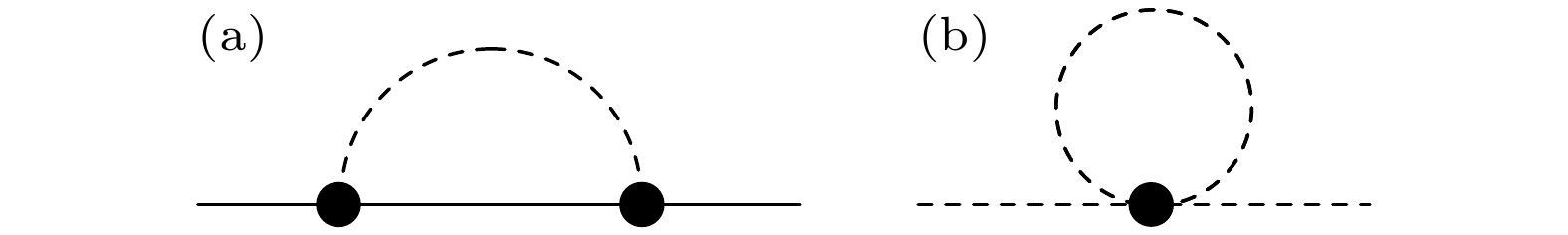
图 1 (a) 八重态重子波函数重整化图; (b) 介子波函数重整化图
Fig. 1. (a) Graph for baryon octet wave function renormalization; (b) graph for pion wave function renormalization.

图 2 衰变s波树图贡献(虚线表示介子, 实线表示重子)
Fig. 2. Tree graph for s-wave hyperon non-leptonic decays (the dotted line denotes meson, and the solid line represents baryon).
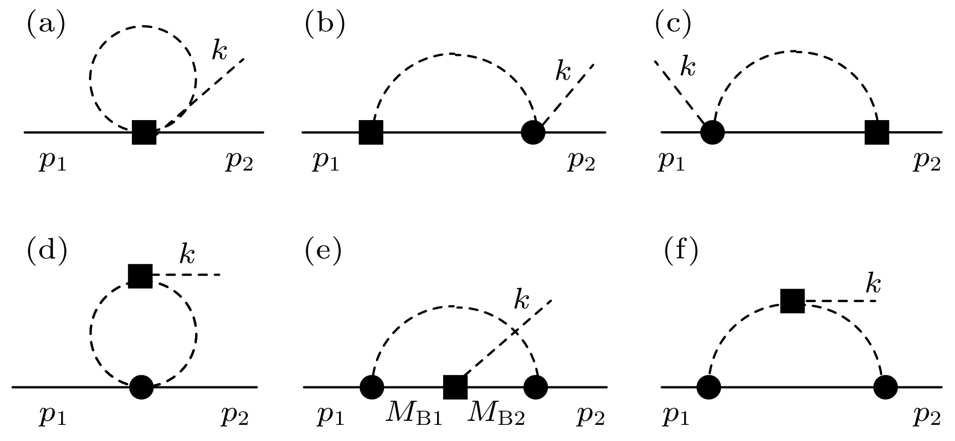
图 3 s波圈图贡献 (黑色方形表示弱作用顶角, 黑色圆形表示强作用)
Fig. 3. One-loop graphs for s-wave hyperon non-leptonic decay amplitudes (the solid square denotes weak interaction vertices, while solid dot represents strong interaction vertices).
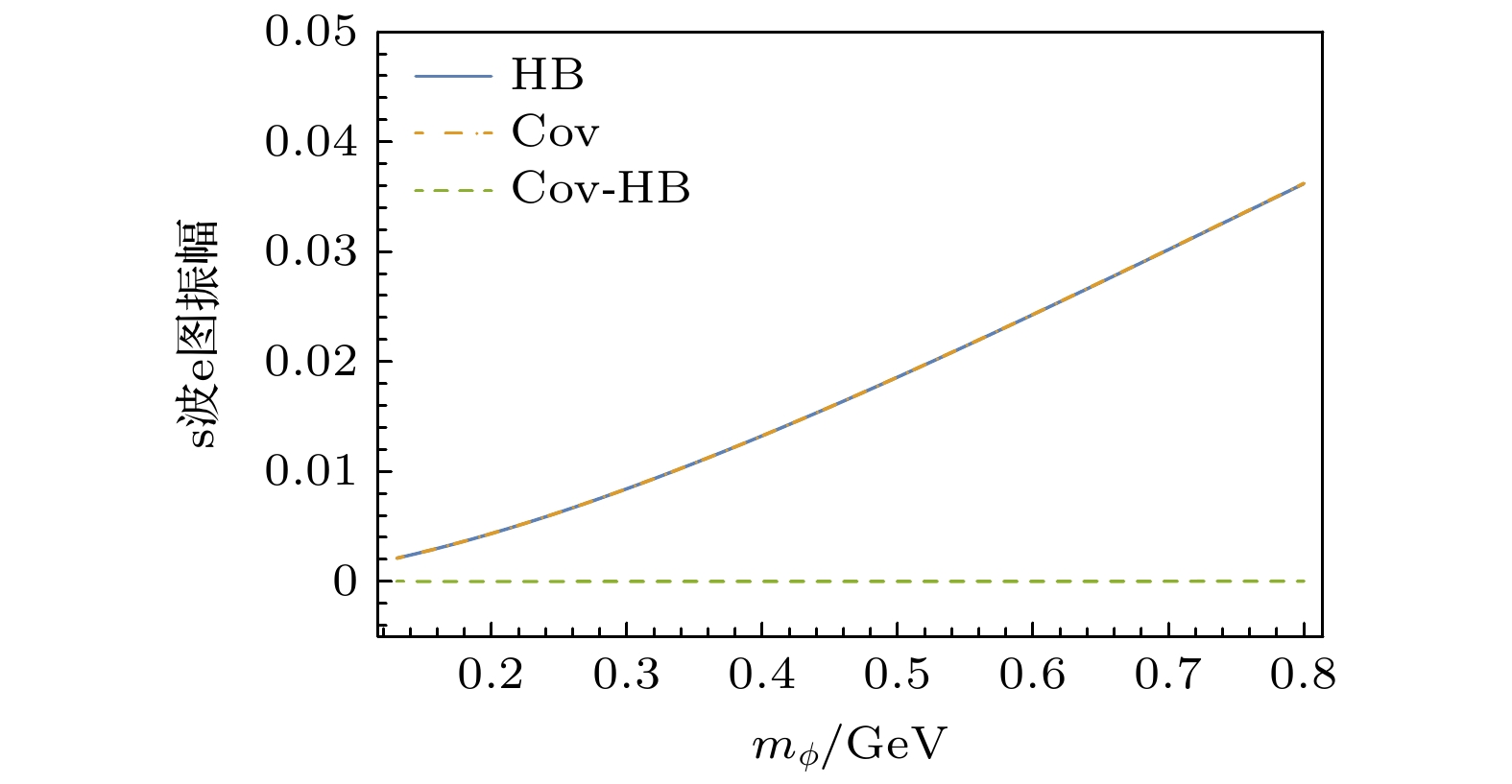
图 6 协变$\varSigma^{({\mathrm{S}}){\mathrm{e}}}_{ij} $与重重子结果的对比
Fig. 6. Comparison of covariant $\varSigma^{({\mathrm{S}}){\mathrm{e}}}_{ij} $ and HB results.
表 1 s波拟合预测s, p波振幅(重整化点: 4πμ2 = 1)
Table 1. Fitting s-wave to predicts s and p wave amplitude (renormalization point: 4πμ2 = 1).
树图 HB(Jenkins) 协变 协变π 协变(π外) 实验 Σ+ → nπ+(s) 0.00 0.02 0.11 0.05 0.06 0.06 ± 0.01 Σ+ → pπ0(s) –1.37 –1.39 –1.60 –0.18 –1.42 –1.38 ± 0.02 Σ– → nπ–(s) 1.94 1.98 2.16 0.36 1.80 1.88 ± 0.01 Λ → pπ–(s) 1.43 1.49 1.58 0.11 1.47 1.38 ± 0.01 Λ → nπ0(s) –1.01 –1.05 –1.19 –0.12 –1.07 –1.03 ± 0.01 Ξ– → nπ–(s) –1.90 –1.76 –1.28 –0.23 –1.05 –1.99 ± 0.01 Ξ0 → nπ0(s) 1.34 1.25 1.03 0.18 0.85 1.51 ± 0.01 Σ+ → nπ+(p) 0.12 0.14 1.03 0.14 0.89 1.81 ± 0.01 Σ+ → pπ0(p) 0.21 0.23 0.72 0.08 0.64 1.24 ± 0.03 Σ– → nπ–(p) –0.18 –0.19 0.02 0.03 –0.01 –0.06 ± 0.01 Λ → pπ–(p) 0.43 1.31 0.38 0.05 0.33 0.63 ± 0.01 Λ → nπ0(p) –0.31 –0.93 –0.27 –0.04 –0.23 –0.41 ± 0.01 Ξ– → nπ–(p) 0.10 –0.21 0.19 0.00 0.19 0.39 ± 0.01 Ξ0 → nπ0(p) –0.07 0.15 –0.14 –0.00 –0.14 –0.27 ± 0.01 hD –0.58 ± 0.09 –0.60 ± 0.12 –0.53 ± 0.35 — — — hF 1.36 ± 0.05 1.00 ± 0.07 0.92 ± 0.20 — — — $ \chi _{1{\text{d}}{\text{.o}}{\text{.f}}}^2 $ 4.15 5.23 1.96 — — — $ \chi _{{\text{2 d}}{\text{.o}}{\text{.f}}}^2 $ 2676.96 3602.73 1403.43 — — —  下载: 导出CSV
表 2 s波拟合预测s, p波振幅(重整化点: 4πμ2 = 4π)
Table 2. Fitting s-wave to predicts s and p wave amplitude (renormalization point: 4πμ2 = 4π).
树图 HB(Jenkins) 协变 协变π 协变(π外) 实验 Σ+ → nπ+(s) 0.00 0.05 0.06 0.25 –0.19 0.06 ± 0.01 Σ+ → pπ0(s) –1.37 –1.39 –1.73 –0.31 –1.42 –1.38 ± 0.02 Σ– → nπ–(s) 1.94 2.02 2.13 0.76 1.37 1.88 ± 0.01 Λ → pπ–(s) 1.43 1.58 1.71 0.08 1.63 1.38 ± 0.01 Λ → nπ0(s) –1.01 –1.12 –1.28 –0.06 –1.22 –1.03 ± 0.01 Ξ– → nπ–(s) –1.90 –1.61 –0.99 –0.35 –0.64 –1.99 ± 0.01 Ξ0 → nπ0(s) 1.34 1.14 0.92 0.25 0.67 1.51 ± 0.01 Σ+ → nπ+(p) 0.12 0.13 1.51 0.18 1.33 1.81 ± 0.01 Σ+ → pπ0(p) 0.21 0.25 1.09 0.10 0.99 1.24 ± 0.03 Σ– → nπ–(p) –0.18 –0.22 –0.03 0.05 –0.08 –0.06 ± 0.01 Λ → pπ–(p) 0.43 0.98 0.33 0.09 0.24 0.63 ± 0.01 Λ → nπ0(p) –0.31 –0.70 –0.23 –0.06 –0.17 –0.41 ± 0.01 Ξ– → nπ–(p) 0.10 –0.36 0.56 0.05 0.51 0.39 ± 0.01 Ξ0 → nπ0(p) –0.07 0.26 –0.40 –0.03 –0.37 –0.27 ± 0.01 hD –0.58 ± 0.09 –0.49 ± 0.12 –0.47 ± 0.31 — — — hF 1.36 ± 0.05 0.71 ± 0.07 0.71 ± 0.19 — — — $ \chi _{1{\text{d}}{\text{.o}}{\text{.f}}}^2 $ 4.15 5.21 1.98 — — — $ \chi _{{\text{2 d}}{\text{.o}}{\text{.f}}}^2 $ 2676.96 3620.78 1556.18 — — —
下载: 导出CSV
表 3 p波拟合预测s, p波振幅(重整化点: 4πμ2 = 1)
Table 3. Fitting p-wave to predicts s and p wave amplitude (renormalization point: 4πμ2 = 1).
树图 HB(Jenkins) 协变 协变π 协变(π外) 实验 Σ+ → nπ+(s) 0.00 0.02 0.22 0.16 0.06 0.06 ± 0.01 Σ+ → pπ0(s) –5.57 –3.31 –2.69 –0.31 –2.38 –1.38 ± 0.02 Σ– → nπ–(s) 7.89 4.70 3.81 0.61 3.20 1.88 ± 0.01 Λ → pπ–(s) 4.01 1.83 2.76 0.24 2.52 1.38 ± 0.01 Λ → nπ0(s) –2.83 –1.29 –2.02 –0.19 –1.83 –1.03 ± 0.01 Ξ– → nπ–(s) –6.83 –3.27 –2.28 –0.41 –1.87 –1.99 ± 0.01 Ξ0 → nπ0(s) 4.83 2.31 1.73 0.30 1.43 1.51 ± 0.01 Σ+ → nπ+(p) 1.45 1.29 1.81 0.25 1.56 1.81 ± 0.01 Σ+ → pπ0(p) 0.87 0.54 1.29 0.14 1.15 1.24 ± 0.03 Σ– → nπ–(p) 0.21 0.53 –0.02 0.05 –0.07 –0.06 ± 0.01 Λ → pπ–(p) 0.74 0.82 0.65 0.09 0.56 0.63 ± 0.01 Λ → nπ0(p) –0.52 –0.58 –0.46 –0.07 –0.39 –0.41 ± 0.01 Ξ– → nπ–(p) 0.84 0.69 0.37 0.00 0.37 0.39 ± 0.01 Ξ0 → nπ0(p) –0.60 –0.49 –0.26 –0.00 –0.26 –0.27 ± 0.01 hD –3.46 ± 0.87 –1.95 ± 0.67 –0.93 ± 0.02 — — — hF 4.43 ± 1.34 1.67 ± 0.62 1.58 ± 0.04 — — — $ \chi _{1{\text{d}}{\text{.o}}{\text{.f}}}^2 $ 98.97 15.57 8.51 — — — $ \chi _{{\text{2 d}}{\text{.o}}{\text{.f}}}^2 $ 71376.35 10276.18 6026.18 — — —
下载: 导出CSV
表 4 p波拟合预测s, p波振幅(重整化点: 4πμ2 = 4π)
Table 4. Fitting p-wave to predicts s and p wave amplitude (renormalization point: 4πμ2 = 4π).
树图 HB(Jenkins) 协变 协变π 协变(π外) 实验 Σ+ → nπ+(s) 0.00 0.05 0.11 0.35 –0.24 0.06 ± 0.01 Σ+ → pπ0(s) –5.57 –3.45 –2.07 –0.38 –1.69 –1.38 ± 0.02 Σ– → nπ–(s) 7.89 4.93 2.66 0.97 1.69 1.88 ± 0.01 Λ → pπ–(s) 4.01 1.99 2.45 0.13 2.32 1.38 ± 0.01 Λ → nπ0(s) –2.83 –1.41 –1.80 –0.09 –1.71 –1.03 ± 0.01 Ξ– → nπ–(s) –6.83 –2.93 –1.37 –0.44 –0.93 –1.99 ± 0.01 Ξ0 → nπ0(s) 4.83 2.07 1.19 0.31 0.88 1.51 ± 0.01 Σ+ → nπ+(p) 1.45 1.43 1.76 0.22 1.54 1.81 ± 0.01 Σ+ → pπ0(p) 0.87 0.60 1.38 0.12 1.26 1.24 ± 0.03 Σ– → nπ–(p) 0.21 0.59 –0.19 0.05 –0.24 –0.06 ± 0.01 Λ → pπ–(p) 0.74 0.83 0.59 0.12 0.47 0.63 ± 0.01 Λ → nπ0(p) –0.52 –0.58 –0.42 –0.08 –0.34 –0.41 ± 0.01 Ξ– → nπ–(p) 0.84 0.38 0.55 0.05 0.50 0.39 ± 0.01 Ξ0 → nπ0(p) –0.60 –0.27 –0.39 –0.03 –0.36 –0.27 ± 0.01 hD –3.46 ± 0.87 –1.46 ± 0.46 –0.51 ± 0.05 — — — hF 4.43 ± 1.34 1.22 ± 0.45 0.96 ± 0.10 — — — $ \chi _{1{\text{d}}{\text{.o}}{\text{.f}}}^2 $ 98.97 16.37 3.41 — — — $ \chi _{{\text{2 d}}{\text{.o}}{\text{.f}}}^2 $ 71376.35 10.647.20 2529.84 — — —
下载: 导出CSV
-
[1] Bijnens J, Sonoda H, Wise M B 1985 Nucl. Phys. B 261 185
Google Scholar
[2] Jenkins E 1992 Nucl. Phys. B 375 561
Google Scholar
[3] Borasoy B, Müller G 2000 Phys. Rev. D 62 054020
Google Scholar
[4] Żenczykowski P 2006 Phys. Rev. D 73 076005
Google Scholar
[5] Le Yaouanc A, Pène O, Raynal J C, Oliver L 1979 Nucl. Phys. B 149 321
Google Scholar
[6] Nardulli G 1988 Nuov. Cim. A 100 485
Google Scholar
[7] Scadron M D, Thebaud L R 1973 Phys. Rev. D 8 2329
Google Scholar
[8] Borasoy B, Holstein B R 1999 Eur. Phys. J. C 6 85
Google Scholar
[9] Borasoy B, Marco E 2003 Phys. Rev. D 67 114016
Google Scholar
[10] Abd El-Hady A, Tandean J 2000 Phys. Rev. D 61 114014
Google Scholar
[11] Becher T, Leutwyler H 1999 Eur. Phys. J. C 9 643
Google Scholar
[12] Fuchs T, Gegelia J, Japaridze G, Scherer S 2003 Phys. Rev. D 68 056005
Google Scholar
[13] Geng L S, Martín Cámalich J, Vicente Vacas M J 2009 Phys. Lett. B 676 63
Google Scholar
[14] Yang J F 2014 Mod. Phys. Lett. A 29 1450043
Google Scholar
[15] Liu Z, Wen L H, Yang J F 2021 Nucl. Phys. B 963 115288
Google Scholar
[16] Fettes N, Meissner U, Steininger S 1998 Nucl. Phys. A 640 199
Google Scholar
[17] Holmberg M, Leupold S 2018 Eur. Phys. J. A 54 103
Google Scholar
[18] Copeland P M, Ji C R, Melnitchouk W 2021 Phys. Rev. D 103 044019
Google Scholar
[19] Jenkins E 1992 Nucl. Phys. B 368 190
Google Scholar
[20] 刘舟, 杨继锋 2022 华东师范大学学报 (自然科学版) 4 103
Google Scholar
Liu Z, Yang J F 2022 J. East China Normal Univ. (Nat. Sci. ) 4 103
Google Scholar
[21] 周海峰, 杨继锋 2024 华东师范大学学报 (自然科学版) 3 12
Google Scholar
Zhou H F, Yang J F 2024 J. East China Normal Univ. (Nat. Sci.) 3 12
Google Scholar
[22] Salone N 2024 Nuov. Cim. 47C 201
[23] Martín Cámalich J, Geng L S,Vicente Vacas M J 2010 Phys. Rev. D 82 074504
Google Scholar
[24] Gell-Mann M 1961 The Eightfold Way: A Theory of strong interaction symmetry Report Number: CTSL-20, TID-12608
[25] Okubo S 1962 Prog. Theo. Phys. 27 949
Google Scholar


 下载:
下载:


计量
- 文章访问数: 936
- PDF下载量: 45
- 被引次数: 0
